import os
import warnings

import contextily as cx
import geopandas as gpd
import igraph as ig
import matplotlib.pyplot as plt
import networkx as nx
import numpy as np
import osmnx as ox
import pandas as pd
from matplotlib.axes import Axes
from matplotlib.colors import LogNorm
from matplotlib.lines import Line2D
from matplotlib.ticker import FuncFormatter, LogLocator

warnings.filterwarnings("ignore")Transport Network Properties
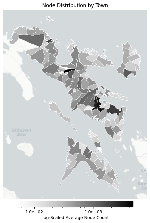
This notebook analyzes the structural properties of the Bicol transport network. It computes node and edge centrality metrics to identify influential points and links, and also detects distinct network communities.
0 Preliminaries
BASE_PATH = "./outputs"
GDF_BOUNDS = gpd.read_file(os.path.join(BASE_PATH, "boundaries.gpkg"))
GRAPH_TRANSPORT = ox.load_graphml(os.path.join(BASE_PATH, "merged_network_simplified.graphml"))
def plot_with_basemap(
ax: Axes,
title: str,
filename: str = None,
padding: float = 0.1,
basemap: bool = True,
) -> None:
if basemap:
x_min, y_min, x_max, y_max = GDF_BOUNDS.total_bounds
ax.set_xlim(x_min - padding, x_max + padding)
ax.set_ylim(y_min - padding, y_max + padding)
cx.add_basemap(
ax,
crs=GDF_BOUNDS.crs,
source=cx.providers.CartoDB.Positron,
attribution="",
)
ax.set_title(title)
ax.set_axis_off()
plt.tight_layout()
if filename:
filepath = os.path.join(BASE_PATH, filename)
plt.savefig(filepath, dpi=300, bbox_inches="tight")
plt.show()
def plot_choropleth(
ax: Axes,
gdf: gpd.GeoDataFrame,
column: str,
title: str,
cmap: str,
filename: str = None,
basemap: bool = True,
cbar: bool = True,
):
data = gdf[column].replace(0, np.nan).dropna()
vmin = max(data.min(), 1e-8)
vmax = data.max()
norm = LogNorm(vmin=vmin, vmax=vmax)
formatter = FuncFormatter(lambda x, _: f"{x:.1e}")
locator = LogLocator(base=10.0, numticks=3)
legend_kwds = {
"label": f"Log-Scaled Average {' '.join(column.split('_')).title()}",
"orientation": "horizontal",
"pad": 0.01,
"shrink": 0.5,
"format": formatter,
"ticks": locator.tick_values(vmin, vmax),
}
gdf.plot(
column=column,
ax=ax,
cmap=cmap,
edgecolor="white",
linewidth=0.5,
legend=cbar,
legend_kwds=legend_kwds,
norm=norm,
)
plot_with_basemap(ax=ax, title=title, filename=filename, basemap=basemap)1 Analyze node distribution
gdf_nodes = ox.graph_to_gdfs(GRAPH_TRANSPORT, edges=False)[["geometry"]]
gdf_nodes = gpd.sjoin(gdf_nodes, GDF_BOUNDS, how="inner", predicate="within")
gdf_nodes = gdf_nodes.drop(columns=["index_right"])
gdf_nodes.head()| geometry | town | province | |
|---|---|---|---|
| osmid | |||
| 300744370 | POINT (124.03376 11.76261) | Esperanza | Masbate |
| 300744933 | POINT (124.06395 11.76468) | Pio V. Corpus | Masbate |
| 300744970 | POINT (124.05778 11.86383) | Pio V. Corpus | Masbate |
| 300745522 | POINT (123.90828 11.91029) | Placer | Masbate |
| 300746507 | POINT (123.99164 11.96455) | Cataingan | Masbate |
def compute_node_counts_by_town(
    gdf_metrics: gpd.GeoDataFrame,
    gdf_nodes: gpd.GeoDataFrame,
    col: str = "node_count",
) -> pd.DataFrame:
    df_node_counts = gdf_nodes.groupby(["town"]).size().reset_index(name=col)
    return gdf_metrics.merge(df_node_counts, on=["town"], how="left")


gdf_metrics = compute_node_counts_by_town(GDF_BOUNDS.copy(), gdf_nodes)
_, ax = plt.subplots(figsize=(8, 8))
plot_choropleth(
ax=ax,
gdf=gdf_metrics,
column="node_count",
title="Node Distribution by Town",
cmap="Greys",
filename="node_count_map.png",
)
def networkx_to_igraph(nx_graph: nx.Graph) -> ig.Graph:
    nx_nodes = list(nx_graph.nodes)
    node_index = {node: idx for idx, node in enumerate(nx_nodes)}

    ig_edges = [(node_index[u], node_index[v]) for u, v in nx_graph.edges()]
    graph = ig.Graph(edges=ig_edges, directed=False)
    graph.vs["name"] = [str(n) for n in nx_nodes]

    return graph, list(node_index.keys())


graph_ig, node_index = networkx_to_igraph(GRAPH_TRANSPORT)
def get_communities(graph: ig.Graph) -> pd.DataFrame:
communities = graph.community_multilevel() # Uses multilevel (Louvain) algorithm
df_communities = pd.DataFrame(
{
"osmid": [int(v["name"]) for v in graph.vs],
"community_id": communities.membership,
}
)
print(f"Detected {len(communities)} communities.")
return df_communities
def plot_communities_map(
gdf_nodes: gpd.GeoDataFrame,
df_communities: pd.DataFrame,
) -> None:
gdf_nodes_w_communities = gdf_nodes.reset_index().merge(df_communities, on="osmid")
_, ax = plt.subplots(figsize=(8, 8))
GDF_BOUNDS.plot(ax=ax, color="none", edgecolor="gray", linewidth=1, zorder=2, alpha=0.5)
gdf_nodes_w_communities.plot(
column="community_id",
categorical=True,
ax=ax,
markersize=3,
cmap="tab20",
zorder=3,
alpha=0.5,
)
plot_with_basemap(
ax=ax,
title="Network Communities in the Bicol Transport System",
filename="network_communities_map.png",
basemap=True,
)
df_communities = get_communities(graph_ig)
plot_communities_map(gdf_nodes, df_communities)Detected 250 communities.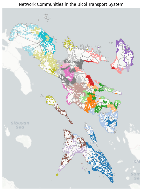
2 Compute centrality metrics for all nodes
try:
    df_centrality = pd.read_csv(os.path.join(BASE_PATH, "node_metrics.csv"))
except FileNotFoundError:
    degree_raw = graph_ig.degree()
    closeness_raw = graph_ig.closeness(normalized=True)
    betweenness_raw = graph_ig.betweenness()

    n = graph_ig.vcount()
    degree_norm = [d / (n - 1) for d in degree_raw]
    betweenness_norm = [b / ((n - 1) * (n - 2)) if n > 2 else 0 for b in betweenness_raw]

    centralities = {
        "osmid": node_index,
        "degree": degree_norm,
        "closeness": closeness_raw,
        "betweenness": betweenness_norm,
    }

    df_centrality = pd.DataFrame(centralities)

df_centrality.head()| osmid | degree | closeness | betweenness | |
|---|---|---|---|---|
| 0 | 300744370 | 0.000053 | 0.003144 | 0.001964 |
| 1 | 300744933 | 0.000053 | 0.003096 | 0.001374 |
| 2 | 300744970 | 0.000053 | 0.003235 | 0.000093 |
| 3 | 300745522 | 0.000053 | 0.003578 | 0.001914 |
| 4 | 300746507 | 0.000053 | 0.003505 | 0.001660 |
df_centrality.to_csv(os.path.join(BASE_PATH, "node_metrics.csv"), index=False)3 Compute average metrics for each town
def get_town_metrics(
gdf_metrics: gpd.GeoDataFrame,
gdf_nodes: gpd.GeoDataFrame,
df_centrality: pd.DataFrame,
) -> gpd.GeoDataFrame:
df_merged = pd.merge(gdf_nodes, df_centrality, on="osmid")
agg_metrics = {"degree": "mean", "betweenness": "mean", "closeness": "mean"}
df_town_metrics = df_merged.groupby(["town"]).agg(agg_metrics).reset_index()
cols = ["town", "province", "degree", "betweenness", "closeness", "geometry"]
return gdf_metrics.merge(df_town_metrics, on=["town"])[cols]
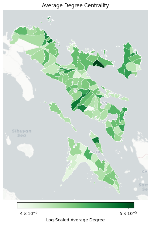
gdf_metrics = get_town_metrics(gdf_metrics, gdf_nodes, df_centrality)_, ax = plt.subplots(figsize=(8, 8))
plot_choropleth(
ax=ax,
gdf=gdf_metrics,
column="degree",
title="Average Degree Centrality",
cmap="Greens",
filename="degree_centrality_map.png",
)
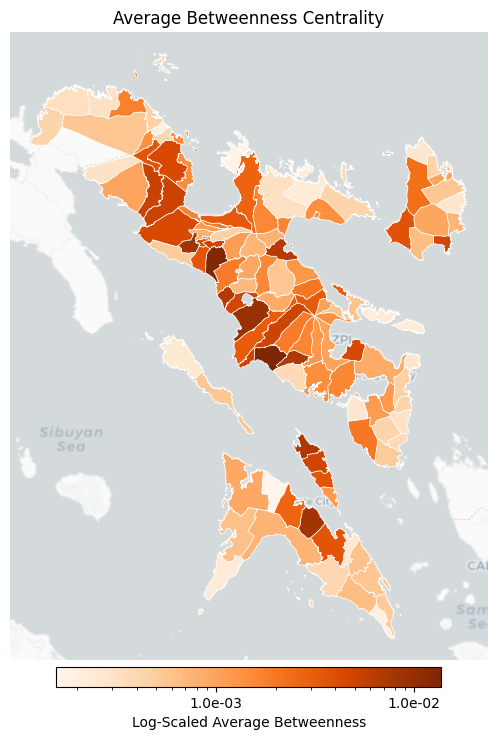
_, ax = plt.subplots(figsize=(8, 8))

plot_choropleth(
    ax=ax,
    gdf=gdf_metrics,
    column="betweenness",
    title="Average Betweenness Centrality",
    cmap="Oranges",
    filename="betweenness_centrality_map.png",
)
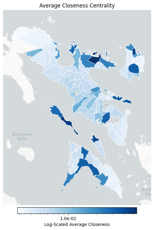
_, ax = plt.subplots(figsize=(8, 8))

plot_choropleth(
    ax=ax,
    gdf=gdf_metrics,
    column="closeness",
    title="Average Closeness Centrality",
    cmap="Blues",
    filename="closeness_centrality_map.png",
)
def get_top_towns_by_centrality(
    gdf_metrics: gpd.GeoDataFrame,
    metric: str,
    top_n: int = 20,
) -> pd.DataFrame:
    return (
        gdf_metrics.nlargest(top_n, metric)[["town", "province", metric]]
        .sort_values(by=metric, ascending=False)
        .reset_index(drop=True)
    )


top_degree_towns = get_top_towns_by_centrality(gdf_metrics, "degree")
top_betweenness_towns = get_top_towns_by_centrality(gdf_metrics, "betweenness")
top_closeness_towns = get_top_towns_by_centrality(gdf_metrics, "closeness")

print("Top Towns by Degree Centrality:")
print(top_degree_towns)

print("\nTop Towns by Betweenness Centrality:")
print(top_betweenness_towns)

print("\nTop Towns by Closeness Centrality:")
print(top_closeness_towns)
Top Towns by Degree Centrality:
town province degree
0 Presentacion Camarines Sur 0.000051
1 Daet Camarines Norte 0.000049
2 Oas Albay 0.000048
3 San Jacinto Masbate 0.000048
4 Vinzons Camarines Norte 0.000048
5 Pio Duran Albay 0.000048
6 Naga City Camarines Sur 0.000047
7 Magarao Camarines Sur 0.000047
8 Panganiban Catanduanes 0.000047
9 Virac Catanduanes 0.000047
10 Santo Domingo Albay 0.000047
11 Prieto Diaz Sorsogon 0.000046
12 Bulusan Sorsogon 0.000046
13 Polangui Albay 0.000046
14 Caramoran Catanduanes 0.000046
15 San Vicente Camarines Norte 0.000046
16 San Andres Catanduanes 0.000046
17 Gubat Sorsogon 0.000046
18 Pandan Catanduanes 0.000046
19 Masbate City Masbate 0.000046
Top Towns by Betweenness Centrality:
town province betweenness
0 Pio Duran Albay 0.013651
1 Minalabac Camarines Sur 0.013362
2 Libon Albay 0.009209
3 Pamplona Camarines Sur 0.008416
4 Mobo Masbate 0.008157
5 Monreal Masbate 0.006978
6 Jovellar Albay 0.006812
7 Balatan Camarines Sur 0.006708
8 Sagñay Camarines Sur 0.006610
9 Lupi Camarines Sur 0.005266
10 Sipocot Camarines Sur 0.005161
11 Milaor Camarines Sur 0.005106
12 Ligao City Albay 0.005086
13 San Jacinto Masbate 0.004947
14 Bato Camarines Sur 0.004718
15 Bato Catanduanes 0.004718
16 Libmanan Camarines Sur 0.004528
17 Basud Camarines Norte 0.004446
18 Manito Albay 0.004393
19 Gainza Camarines Sur 0.004307
Top Towns by Closeness Centrality:
town province closeness
0 Garchitorena Camarines Sur 0.055026
1 Claveria Masbate 0.047951
2 Bagamanoc Catanduanes 0.042953
3 Monreal Masbate 0.042692
4 Rapu-Rapu Albay 0.034115
5 Milagros Masbate 0.032388
6 San Miguel Catanduanes 0.032173
7 Castilla Sorsogon 0.031637
8 Baleno Masbate 0.030605
9 Siruma Camarines Sur 0.029557
10 San Pascual Masbate 0.028352
11 Balud Masbate 0.021489
12 Caramoan Camarines Sur 0.021380
13 Lagonoy Camarines Sur 0.020998
14 Pandan Catanduanes 0.019475
15 Cawayan Masbate 0.019248
16 Malinao Albay 0.017879
17 Mercedes Camarines Norte 0.016397
18 Panganiban Catanduanes 0.016139
19 Oas Albay 0.0126444 Analyze edge metrics
def get_edge_betweenness(nx_graph: nx.Graph, ig_graph: ig.Graph) -> gpd.GeoDataFrame:
    _, gdf_edges = ox.graph_to_gdfs(nx_graph)

    edge_betweenness_raw = ig_graph.edge_betweenness()

    n = ig_graph.vcount()
    if n > 2:
        normalizing_factor = (n * (n - 1)) / 2
        edge_betweenness_norm = [b / normalizing_factor for b in edge_betweenness_raw]
    else:
        edge_betweenness_norm = [0] * len(edge_betweenness_raw)

    gdf_edges["edge_betweenness"] = edge_betweenness_norm

    print(f"Computed edge betweenness for {len(gdf_edges)} edges.")
    return gdf_edges


def plot_edge_betweenness_map(gdf_edges: gpd.GeoDataFrame) -> None:
    criticality_percentile = 0.99
    betweenness_threshold = gdf_edges["edge_betweenness"].quantile(criticality_percentile)
    gdf_critical_edges = gdf_edges[gdf_edges["edge_betweenness"] >= betweenness_threshold]

    print(
        f"Identified {len(gdf_critical_edges)} critical edges (top {100 - criticality_percentile*100:.1f}%) "
        f"with betweenness >= {betweenness_threshold:.6f}"
    )

    _, ax = plt.subplots(figsize=(10, 10))

    gdf_edges.plot(ax=ax, linewidth=0.5, edgecolor="#d3d3d3", zorder=2)
    gdf_critical_edges.plot(ax=ax, linewidth=1.5, edgecolor="crimson", zorder=3)
    GDF_BOUNDS.plot(ax=ax, color="none", edgecolor="black", linewidth=1.0, zorder=4, alpha=0.6)
    cx.add_basemap(ax, crs=gdf_edges.crs, source=cx.providers.CartoDB.Positron, attribution="", zorder=1)

    legend_elements = [
        Line2D([0], [0], color="#d3d3d3", lw=1, label="Transport Network"),
        Line2D(
            [0],
            [0],
            color="crimson",
            lw=2,
            label=f"Critical Edges (Top {100-criticality_percentile*100:.1f}%)",
        ),
        Line2D([0], [0], color="black", lw=1, label="Town Boundaries"),
    ]
    ax.legend(handles=legend_elements, loc="upper right")

    ax.set_title("Critical Transport Links by Edge Betweenness Centrality", fontsize=14)
    ax.set_axis_off()
    plt.tight_layout()

    filepath = os.path.join(BASE_PATH, "edge_betweenness_map.png")
    plt.savefig(filepath, dpi=300, bbox_inches="tight")
    plt.show()


gdf_edges_centrality = get_edge_betweenness(GRAPH_TRANSPORT, graph_ig)
plot_edge_betweenness_map(gdf_edges_centrality)
Computed edge betweenness for 71895 edges.
Identified 719 critical edges (top 1.0%) with betweenness >= 0.065309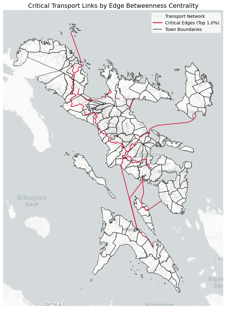
# --- Code Cell 16 ---
def get_critical_edges(gdf_edges: gpd.GeoDataFrame) -> gpd.GeoDataFrame:
    """Filters edges to include only those considered 'critical' based on a percentile."""
    criticality_percentile = 0.99
    betweenness_threshold = gdf_edges["edge_betweenness"].quantile(criticality_percentile)
    return gdf_edges[gdf_edges["edge_betweenness"] >= betweenness_threshold]


def count_critical_edges_by_town(
    gdf_critical_edges: gpd.GeoDataFrame, gdf_boundaries: gpd.GeoDataFrame
) -> pd.DataFrame:
    """Counts the number of critical edges within each town by performing a spatial join."""
    # The sjoin operation finds which town each edge intersects with
    gdf_located_edges = gpd.sjoin(gdf_critical_edges, gdf_boundaries, how="inner", predicate="intersects")

    # Group by both province and town, then count the number of edges
    df_counts = gdf_located_edges.groupby(["province", "town"]).size().reset_index(name="critical_edge_count")

    # Sort the results to find the towns with the most critical edges
    df_counts = df_counts.sort_values(by="critical_edge_count", ascending=False)

    return df_counts


# Identify critical edges from the centrality analysis
gdf_critical_edges = get_critical_edges(gdf_edges_centrality)

# Count the critical edges per town and include the province
df_critical_edge_counts = count_critical_edges_by_town(gdf_critical_edges, GDF_BOUNDS)

# Print the top 20 results
print("--- Top 20 Towns with Most Critical Edges ---")
print(df_critical_edge_counts.head(20).to_string(index=False))
--- Top 20 Towns with Most Critical Edges ---
province town critical_edge_count
Albay Ligao City 62
Albay Tabaco City 54
Camarines Sur Libmanan 53
Camarines Norte Basud 49
Camarines Sur Minalabac 38
Masbate Mobo 38
Albay Pio Duran 35
Albay Daraga 32
Camarines Sur Pamplona 31
Camarines Sur San Fernando 30
Camarines Sur Sipocot 26
Albay Libon 23
Camarines Sur Lupi 22
Camarines Sur Calabanga 20
Masbate Uson 19
Camarines Sur Tinambac 19
Masbate Monreal 18
Albay Legazpi City 18
Masbate San Jacinto 17
Camarines Sur Bato 17